Module 10: Building a Package with R-Studio
--March 17th, 2021--
This week's assignment required the creation of a test package to learn the basic process of creating a package using
R-Studio, and to fill out the test package's description file.
The videos and readings posted on Canvas were very helpful, and the overall assignment went smoothly.
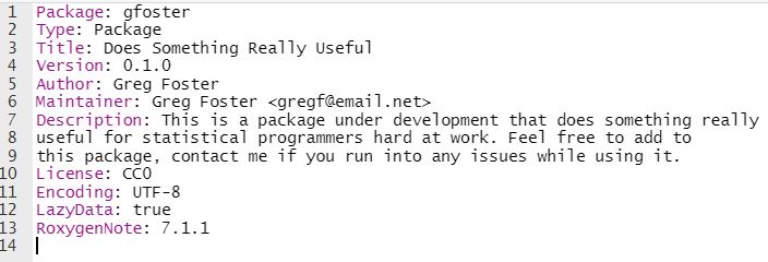
I created a test package named "gfoster", with a single function named "goodbye" that takes one parameter, x, and prints out the
message "Goodbye x, nice to see you!". The description file can be seen below. It is filled with gibberish for the sake of
the example, please don't think this is my attempt at a real package haha.
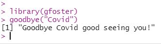
 An example of the package being loaded and used in R is below.
 As always, all of the files can be found on my Github page. The description file can
be located in the "gfoster" folder, and should have a commit comment of "module 10 update 3".
As always, all of the files can be found on my Github page. The description file can
be located in the "gfoster" folder, and should have a commit comment of "module 10 update 3".
Module 09: Visualizations with R
--March 13th, 2021--
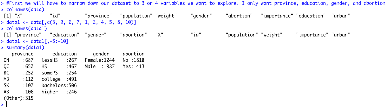
This week's assignment was all about exploring different types of data visualizations in R. I decided to use the 2011 Canadian Election survey data regarding abortion sentiment. A short snippet of the dataset can be seen below:
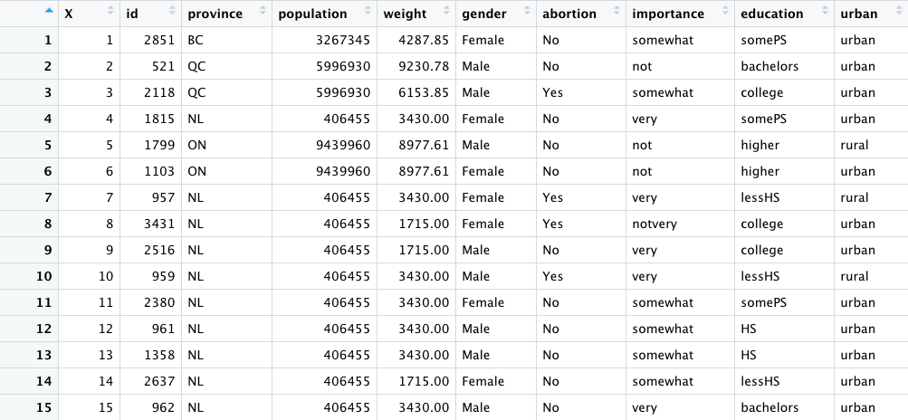 The columns I decided to focus on were province, gender, abortion sentiment, education, and urban. The province column
indicates which Canadian province the voter lived in. The abortion column indicates whether the voter thinks that abortions should be banned in Canada.
"No" signifies that the voter does NOT want abortion to be banned, and "Yes" signifies that the voter DOES want abortion to be banned.
The education column indicates the highest level of education achieved by the voter, and the urban column indicates whether the voter lived in an "urban" or
"rural" region of their respective province.
The columns I decided to focus on were province, gender, abortion sentiment, education, and urban. The province column
indicates which Canadian province the voter lived in. The abortion column indicates whether the voter thinks that abortions should be banned in Canada.
"No" signifies that the voter does NOT want abortion to be banned, and "Yes" signifies that the voter DOES want abortion to be banned.
The education column indicates the highest level of education achieved by the voter, and the urban column indicates whether the voter lived in an "urban" or
"rural" region of their respective province.
After loading the data into R as a CSV file, I used the class() and summary() functions to take a quick look at the dataset.
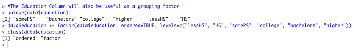
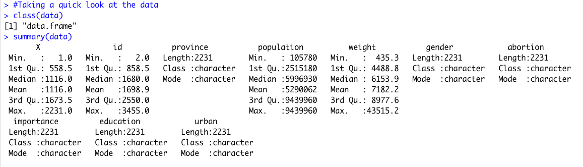 The data object is registered as a data frame, so that is good, however many of the columns I wanted to analyze were in character format. To fix This
I used the unique() and factor() functions to turn the character columns into ordered factors. An example with the education column is below:
The data object is registered as a data frame, so that is good, however many of the columns I wanted to analyze were in character format. To fix This
I used the unique() and factor() functions to turn the character columns into ordered factors. An example with the education column is below:
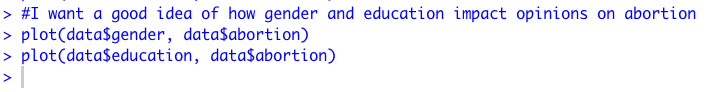
 With the desired columns formatted as ordered factors, I was able to start exploring the dataset with visualizations.
I started with base R graphics, comparing gender to abortion and then education to abortion with the plot() function.
With the desired columns formatted as ordered factors, I was able to start exploring the dataset with visualizations.
I started with base R graphics, comparing gender to abortion and then education to abortion with the plot() function.
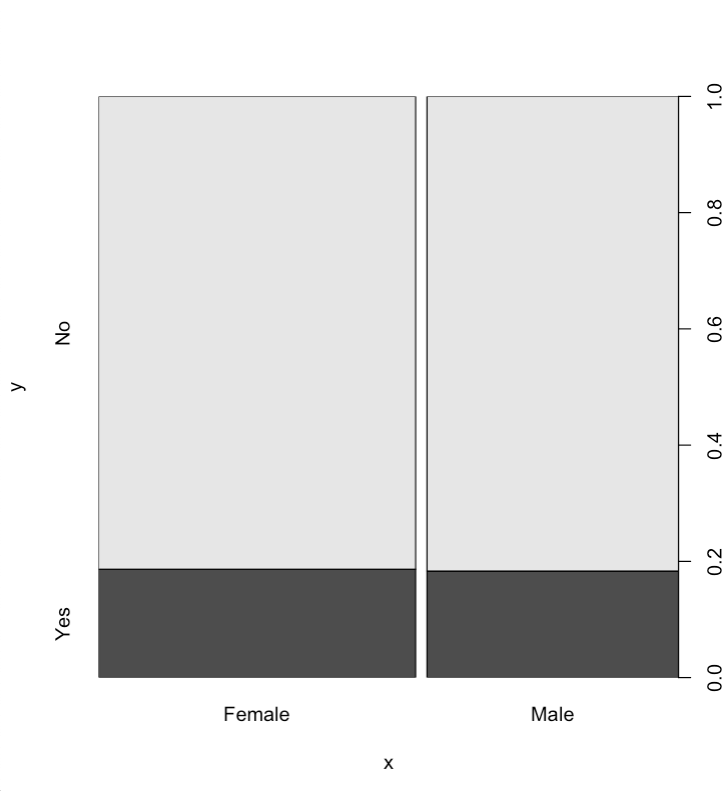 It looks like gender doesn't play a huge role, the vast majority of people regardless of gender feel that abortion should not be banned.
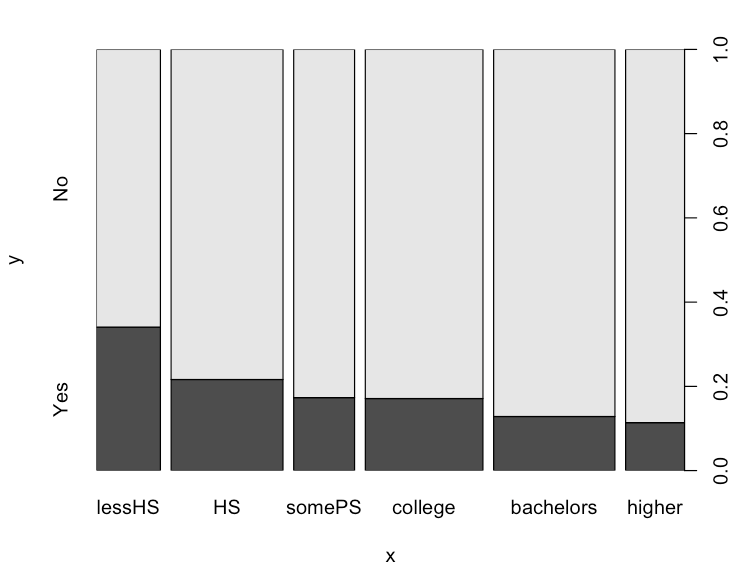 The education plot reveals an interesting trend, as the highest educated population, those with a graduate degree ("higher"), has the lowest percentage of people that think abortion should be banned.
Similarly, the least educated population, those that didn't finish high school, has the highest population of people that think abortions should be banned.
The education plot reveals an interesting trend, as the highest educated population, those with a graduate degree ("higher"), has the lowest percentage of people that think abortion should be banned.
Similarly, the least educated population, those that didn't finish high school, has the highest population of people that think abortions should be banned.
With some initial data exploration with base R graphics, I then turned to the ggplot2 package for visualizations. I first plotted provinces vs abortion sentiment, colored by abortion sentiment with geom_col().

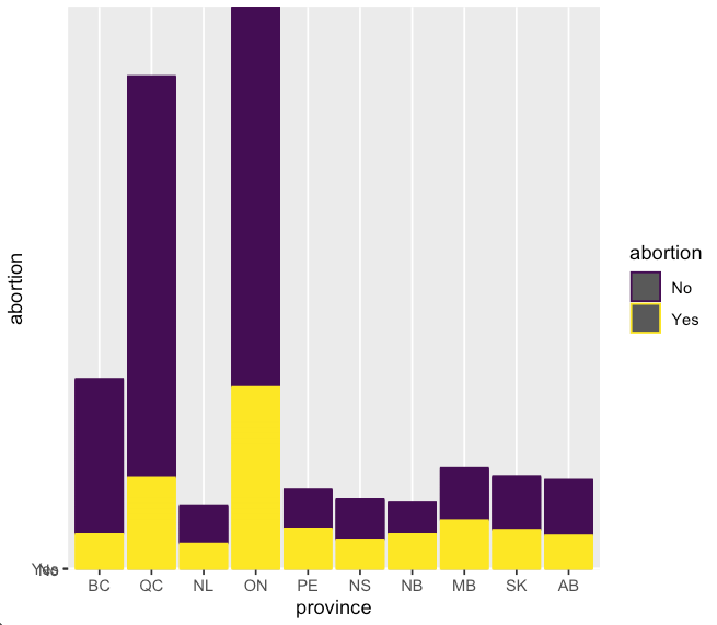 It looks like Ontario and Quebec have the highest populations in favor of abortion being banned, highlighted in yellow. This being said, these two provinces
are also very highly populated, and the overall proportion of pro-abortion vs anti-abortion weighs strongly in favor of pro-abortion.
It looks like Ontario and Quebec have the highest populations in favor of abortion being banned, highlighted in yellow. This being said, these two provinces
are also very highly populated, and the overall proportion of pro-abortion vs anti-abortion weighs strongly in favor of pro-abortion.
I was also interested to know if urban vs rural populations would vote differently regarding abortion.

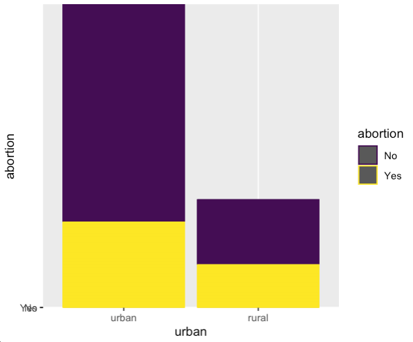 It appears that the urban populations have more people overall in favor of getting rid of abortions, however this is a relatively small portion of the urban population overall.
The rural population, on the other hand, is split roughly 40-60 on the abortion debate, with the majority voting "No" to banning abortion. It makes sense that the rural population has
a higher proportion of anti-abortion sentiment, given that rural areas tend to vote more conservatively than urban areas.
It appears that the urban populations have more people overall in favor of getting rid of abortions, however this is a relatively small portion of the urban population overall.
The rural population, on the other hand, is split roughly 40-60 on the abortion debate, with the majority voting "No" to banning abortion. It makes sense that the rural population has
a higher proportion of anti-abortion sentiment, given that rural areas tend to vote more conservatively than urban areas.
Now that base R and ggplot2 have been explored to an extent, I moved on to producing a multivariate plot to enable the comparison of 3 or more variables
simultaneously. Before using the cdparcoord package to produce an interactive visualization, I first re-ordered the dataset columns and removed all but the province, education, gender, and abortion columns.
 Once the data1 object was prepared for visualization, I went ahead and used the discretize() and discparcoord() functions to produce the visualization seen below.

The visualization loads with all of the possible values selected, but playing around with de-selecting certain parameters lets you see the impact on the end lines pointing to either "yes" or "no" regarding banning abortion. A deep blue line pointing to "No" indicates that over 80 voters
fitting the selected parameters felt that abortion should NOT be banned. A deep blue line pointing to "Yes" means the opposite. Red lines generally indicate that very few voters made a particular decision, while lines colored somewhere inbetween red and blue indicate that somewhere between
30 and 50 voters made that particular decision.
Manipulating the province and education values within the visualization also provide insight into which provinces have higher proportions of well-educated voters. Quebec and Ontario both stand out as having more graduate level voters than the other provinces.
Overall, I think the most useful visualization was the bar-chart showing voter abortion sentiment by province, colored by abortion sentiment. A quick look at this
visualization makes it easy to see that Canadian voters as a whole voted predominantly to keep abortion, particularly in highly populated provinces. It is also easy to see that the lower populated provinces, which are likely to be more rural and therefore conservative, were more evenly divided on the issue.
If the highly populated Ontario, Quebec, and British Columbia provinces were removed from the vote, it would be a tough call on which side of the abortion argument would win.
This was an interesting assignment, and I enjoyed exploring the chosen data with different visualization approaches.
As always, all of the files can be found on my Github page.
Module 08: Reading and Manipulating Datasets in txt formats with plyr
--March 7th, 2021--
This week's assignment required the reading and manipulation of a dataset in a .txt format, which I have never done before. It ended up being really simple, especially with the provided instructions.
I enjoyed using the plyr package, and learning about it's immense utility in manipulating and summarizing dataframes. I can see a lot of potential uses for this package in the final project.
I documented the overall process in the compiled R markdown file below. Due to the laid-back nature of this week's homework, I decided to add a small challenge by formatting the output file to look more professional.
All of the files can be found on my Github page.
Module 07: S3 and S4 Object-Oriented Programming in R
--February 27th, 2021--
This week's module was very interesting, I enjoy using the OOP S3 and S4 systems and am excited to see how
they can be used to supplement data analysis and package creation.
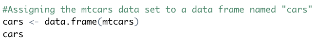
I decided to use the mtcars data set, included in R by default. I assigned it to a data frame
named "cars" for convenience.
 Next I used some generic S3 functions on the dataset.
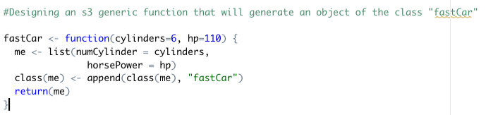
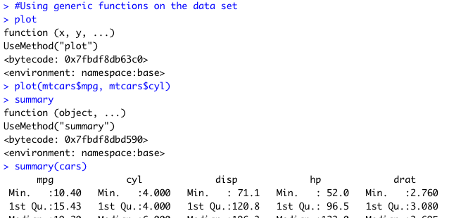 I then created a function "fastCar" to create objects using data from the mtcars data set of the class "fastCar".
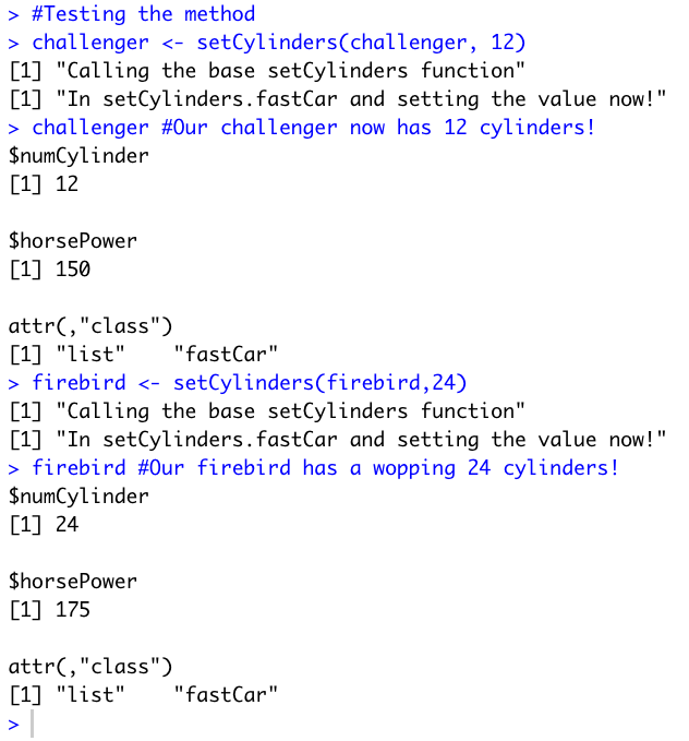
 I created two objects for this class using the function.
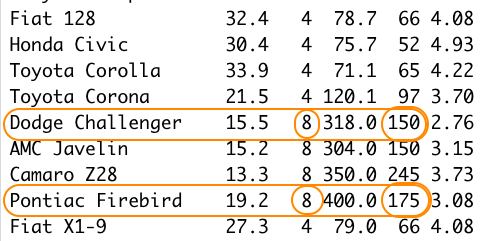
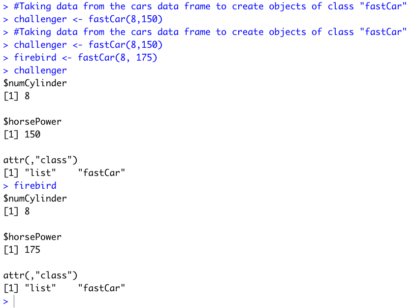 You can see that both of these objects are of class "fastCar", and checking with the mtcars data set, you can see
that these objects correctly represent the two cars named "Dodge Challenger" and "Pontiac Firebird".
You can see that both of these objects are of class "fastCar", and checking with the mtcars data set, you can see
that these objects correctly represent the two cars named "Dodge Challenger" and "Pontiac Firebird".
 Next I created a method for this S3 class to change the number of cylinders assigned to objects.
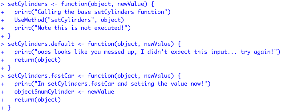 It required the creation of three different functions. A generic function with the required "UseMethod" function embedded within it, a default function to run when
R can't locate a proper class to run the function on, and a function telling R what to do when the generic function is called on an object of class "fastCar".
It required the creation of three different functions. A generic function with the required "UseMethod" function embedded within it, a default function to run when
R can't locate a proper class to run the function on, and a function telling R what to do when the generic function is called on an object of class "fastCar".
I then used the new class method "setCylinders" on the two previously created S3 objects "Challenger" and "Firebird" to give them a ridiculous number of engine cylinders.
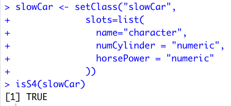
 Moving on to S4 classes and objects, I defined a function that generates objects of the class "slowCar". I also checked to make sure this function was considered to be S4, using the
isS4() function.
Moving on to S4 classes and objects, I defined a function that generates objects of the class "slowCar". I also checked to make sure this function was considered to be S4, using the
isS4() function.
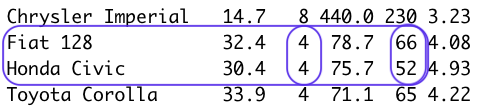
 I then used the new() function to create two new objects of the newly defined "slowCar" class. I chose the "Fiat 128" and "Honda Civic" cars from the mtcars data set.
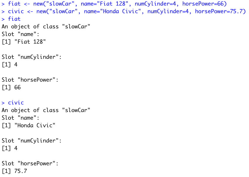 Once again checking with the mtcars dataset, you can see that the names, number of cylinders, and horsepower are all accurate.
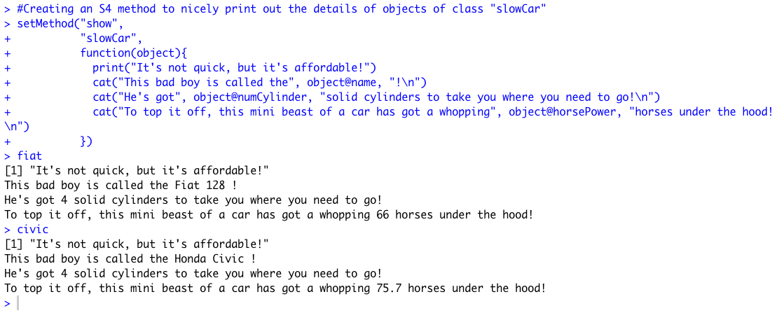
 I then defined a method for this S4 class "slowCar" for the generic "show()" function that operates in the background whenever the name of an object is typed into the console.
I proceeded to test the method with the two created objects "fiat" and "civic". The function prints out the details of each object in nicely formatted sentences.
I then defined a method for this S4 class "slowCar" for the generic "show()" function that operates in the background whenever the name of an object is typed into the console.
I proceeded to test the method with the two created objects "fiat" and "civic". The function prints out the details of each object in nicely formatted sentences.
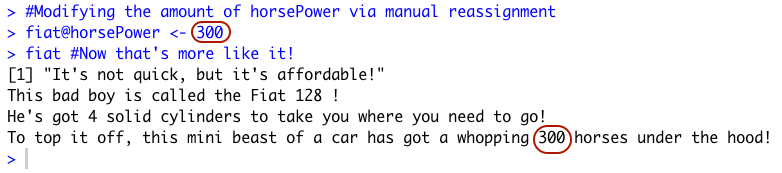
 Next I tried manual reassignment of the "horsePower" slot for the "fiat" object, making it's horsepower 300.
Now to answer the four questions posed in the assignment on Canvas.
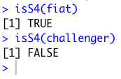
1. You can tell what object-oriented system an object is associated with by using the isS4() function,
with the object in question as the argument. I tested the S3 object "challenger" and the S4 object "fiat" with the
function. Remember that the "challenger" object was created with an S3 function, and the "fiat" object was created with an S4 function.
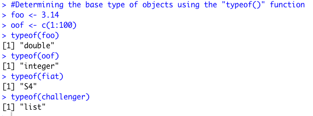
 2. You can determine the base type of an object using the "typeof()" function in R. Some examples are below. Notice that the
"fiat" object is considered S4, while the "challenger" object is considered a "list", not S3.
2. You can determine the base type of an object using the "typeof()" function in R. Some examples are below. Notice that the
"fiat" object is considered S4, while the "challenger" object is considered a "list", not S3.
 3. A generic function in R is like a multi-purpose operator that changes how it works depending on what class of object it is faced with.
It can be altered to use an unlimited number of different objects, as long as it has instructions on how to use each object. In this week's assignment,
generic functions were used multiple times.
3. A generic function in R is like a multi-purpose operator that changes how it works depending on what class of object it is faced with.
It can be altered to use an unlimited number of different objects, as long as it has instructions on how to use each object. In this week's assignment,
generic functions were used multiple times.
In the S3 examples, I defined a new generic function that only knows how to use one class of objects, "fastCar". This
generic function can be expanded upon to use other classes of objects if needed. In the S4 example, I added a method to the generic function "show()" to tell the
function exactly what to do when using an object of class "slowCar".
4. The main differences between S3 and S4 object oriented programming in R : S4 classes are formally defined, and objects associated with them are classified in R as belonging to them.
Objects associated with S3 classes are recognized by R as lists with an attribute of the S3 class. S4 has something called "multiple dispatch", which allows the generic functions to determine which
methods to use based on multiple arguments, rather than S3, which only views the first argument of a generic function to determine which method to use.
This results in fewer user errors when using a package written with S4 classes and methods.
All-in-all, S4 is a more stable format for creating packages in R.
This last question was tricky, I used this webpage for help:
As always the compiled R file can be found below, and all of the files can be found on my Github page.
Module 06: More Matrices in R
--February 19th, 2021--
The readings this week were interesting, I enjoyed learning the overall process of creating an R package. The introduction to object-oriented programming in R with the differences
between S3 and S4 was cool as well.
This week's assignment was fairly simple, I found the diag() function in R to be very straight forward. Adding and subtracting matrices was also much easier to understand than
multiplying them.
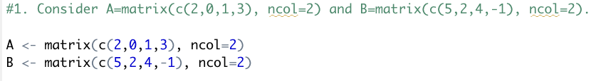
Question 1 first required the creation of two square matrices.
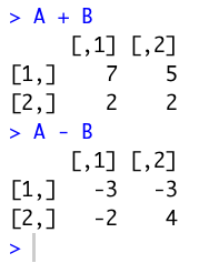
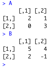 Then some simple addition and subtraction operations with the newly created matrices.
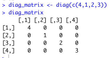
 Question 2 required the creation of a 4 column, 4 row matrix with the values 4,1,2,3 in the diagonal, using the diag() function.
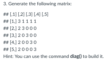
 Question 3 required the creation of a 5 column, 5 row matrix with 3's filling up the diagonal, 2's filling up the rest of the first column, and 1's filling up the rest of the first row.
The example provided is below:
Question 3 required the creation of a 5 column, 5 row matrix with 3's filling up the diagonal, 2's filling up the rest of the first column, and 1's filling up the rest of the first row.
The example provided is below:
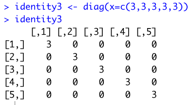
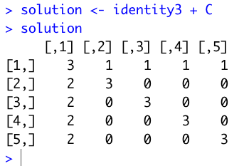
 I first generated a 5x5 identity matrix with 3's in the diagonal using the diag() function.
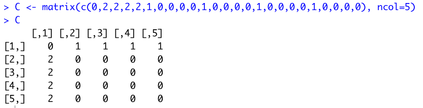
 I then created another 5x5 matrix, this time with zeros everywhere except the 1's and 2's required in the first row and first column.
I used matrix(c(0,2,2,2,2,1,0,0,0,0,1,0,0,0,0,1,0,0,0,0,1,0,0,0,0), ncol=5).
I then created another 5x5 matrix, this time with zeros everywhere except the 1's and 2's required in the first row and first column.
I used matrix(c(0,2,2,2,2,1,0,0,0,0,1,0,0,0,0,1,0,0,0,0,1,0,0,0,0), ncol=5).
 Finally I added the two matrices together, getting the desired result.
As always the compiled R file can be found below, and all of the files can be found on my Github page.
Module 05: Matrices in R
--February 14th, 2021--
This assignment focused on learning about using matrices in R programming. The initial task was to
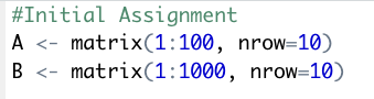
find the inverse and determinant of two matrices named A and B. A was a 10 column, 10 row matrix with values from
1 to 100. B was a 10 row, 100 column matrix with values from 1 to 1000.
I generated the two matrices using the matrix() function in R, assigning them to variables A and B.
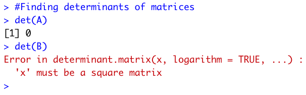
 I then found the determinants for both matrices using the det() function in R. The determinant of A was
0, and the determinant of B couldn't be found because it was a non-square matrix.
I then found the determinants for both matrices using the det() function in R. The determinant of A was
0, and the determinant of B couldn't be found because it was a non-square matrix.
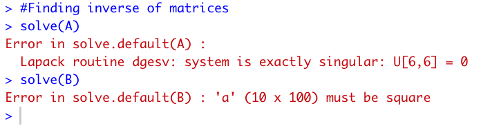
 I then used the solve() function in R to find the inverse values of the two matrices. Matrix A did not have an inverse
because it was "exactly singular", and matrix B did not have a clear inverse once again because it was non-square.
I then used the solve() function in R to find the inverse values of the two matrices. Matrix A did not have an inverse
because it was "exactly singular", and matrix B did not have a clear inverse once again because it was non-square.
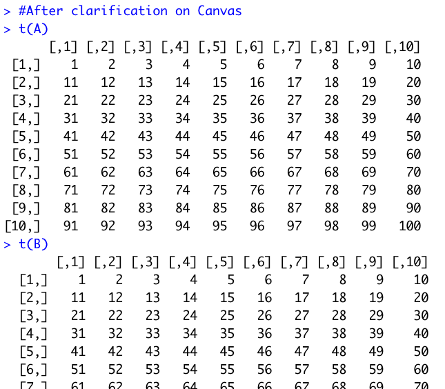
 In the second portion of the assignment outlined in the Announcement on Canvas, several matrix calculations were required.
Using the same matrices, A and B, the first step was transposing them using the t() function in R.
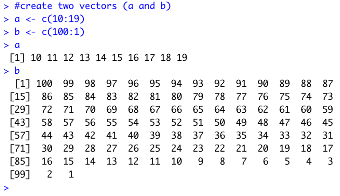
 The next step was to create two vectors. I purposefully made sure that each vector, a and b, had either 10 or 100 values
so that they would better align with matrices A and B for multiplication using the %*% argument.
The next step was to create two vectors. I purposefully made sure that each vector, a and b, had either 10 or 100 values
so that they would better align with matrices A and B for multiplication using the %*% argument.
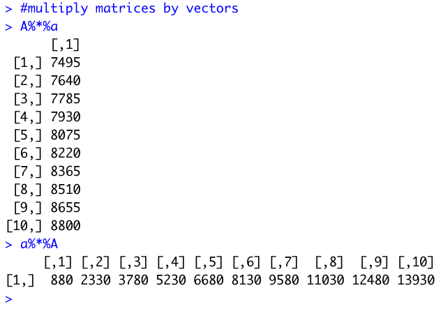
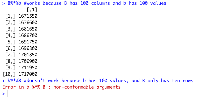
 Next we had to test matrix multiplication using the %*% argument with matrices A and B, and vectors a and b.
Matrix A and vector a were able to be multiplied in any order, since the length of vector a is 10 and matrix A has both 10
columns and 10 rows.
Next we had to test matrix multiplication using the %*% argument with matrices A and B, and vectors a and b.
Matrix A and vector a were able to be multiplied in any order, since the length of vector a is 10 and matrix A has both 10
columns and 10 rows.
 Matrix B and vector b could only be multiplied without error when matrix B was placed before vector b. This is because matrix B has the same number of columns, 100, as vector b has values, also 100.
When vector b comes before matrix B in the calculation (b %*% B), R returns an error because the values of vector b don't equal the number of rows in matrix B, which is 10.
Matrix B and vector b could only be multiplied without error when matrix B was placed before vector b. This is because matrix B has the same number of columns, 100, as vector b has values, also 100.
When vector b comes before matrix B in the calculation (b %*% B), R returns an error because the values of vector b don't equal the number of rows in matrix B, which is 10.
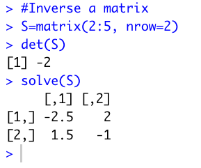
 The final task was finding the inverse of a square matrix with two columns, two rows, and values 2 through 5. The matrix was generated using the matrix() function
in R, the determinant was found with the det() function, and the inverse was found with the solve() function.
The final task was finding the inverse of a square matrix with two columns, two rows, and values 2 through 5. The matrix was generated using the matrix() function
in R, the determinant was found with the det() function, and the inverse was found with the solve() function.
 Before this assignment I was very unfamiliar with matrices, so this was a good help in learning the basics of their use and general terminology. I ended up reading about matrix multiplication
online to understand what exactly the computer is doing when using the %*% argument, as I was not previously exposed to matrices in any math classes prior to this course.
Before this assignment I was very unfamiliar with matrices, so this was a good help in learning the basics of their use and general terminology. I ended up reading about matrix multiplication
online to understand what exactly the computer is doing when using the %*% argument, as I was not previously exposed to matrices in any math classes prior to this course.
Looking forward to progressing towards building an R package!
As always the compiled R file can be found below, and all of the files can be found on my Github page.
Module 04: Blood Pressure Diagnoses
--February 1st, 2021--
This week's assignment required the analysis of some sample medical data representing blood pressure diagnoses of 10 different patients.
Two side by side plots were required. The assignment wanted a histogram next to a boxplot, and for these plots to visualize firstly the patient blood pressure
and then the medical doctor's final decision regarding their need for immediate care. I found that the most meaningful way to organize the plots was by comparing
the histogram of blood pressure to the histogram of final decision, and likewise for the box plots.
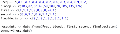
I first created numeric vectors with the supplied data, with help from the assignment's hint. I then combined the vectors into a dataframe named "hosp_data".
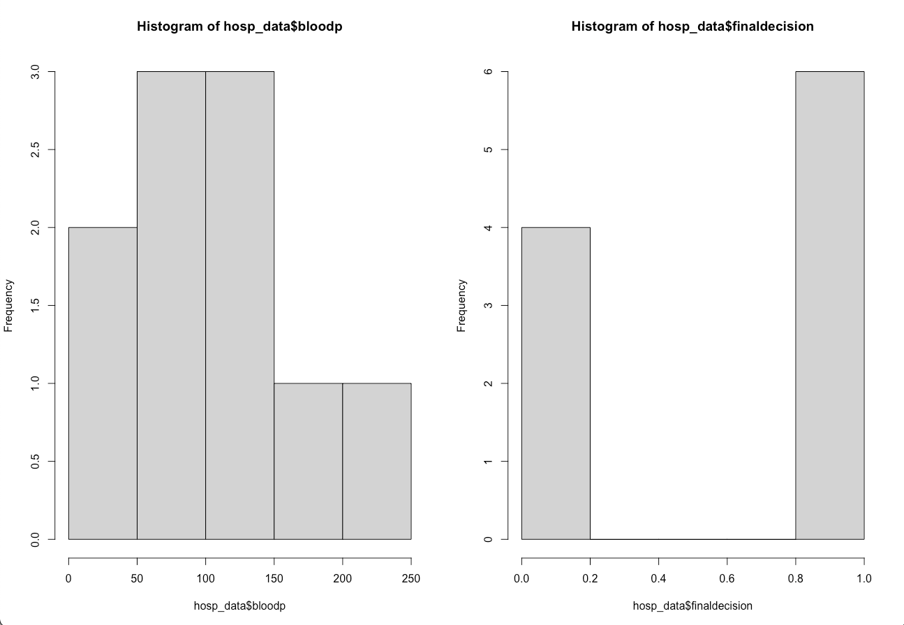
 I then generated a side by side plot using "par(mfrow=c(1,2)", placing the histograms for blood pressures and final decision together for comparison.
 Next I generated a side by side plot placing the box plots for blood pressure and final decision next to eachother.
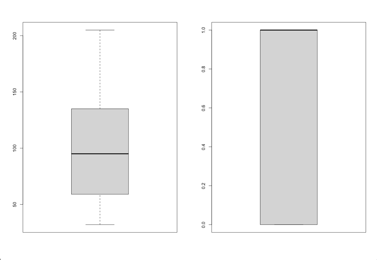 The histograms ended up being far more useful for data comparison than the box plots, as you are able to see the different distributions of the data more effectively.
From the side by side histograms you can see that the relationship between patient blood pressure and final decision for care by a medical doctor appear to make sense.
6 patients received high priority for immediate medical care. Four of the patient blood pressures stand out as being very abnormal and dangerous. Two patients had blood pressures
under 50, indicating severe hypotension, while two other patients had blood pressures over 150, indicating cardiovascular hypertension. The other two patients that received immediate care
may have had relatively normal blood pressures but other health variables not recorded led to the doctor's final decision.
The information presented is not nearly enough to make an informed decision as to the efficacy and accuracy of the medical doctor's diagnoses. For one there are only
10 patients presented in the dataset, and in order to properly gauge the efficacy of a diagnosis we need data on the patient's other health markers, like blood content levels,
body temperature, heart rate, and general condition.
As always the compiled R file can be found below, and all of the files can be found on my Github page.
Module 03: Matrices and Data Frames
--January 26th, 2021--
This week's module was difficult. I continuously ran into errors with the prescribed operations in the assignment. While I worked around some of them, I was unable to complete
certain portions due to these unrelenting errors.
The most challenging portion was the matrix multiplication, as attempting to multiply a matrix is impossible to my knowledge with the dataset provided, unless the names column is taken away in order for the
matrix to recognize the numbers as integers. With this in mind, I attempted to recreate the example provided in the assignment, but could not for the life of me figure out how to make as.matrix(C.df)%*%B produce
anything other than errors. The error I kept receiving is shown below:

I did end up successfully obtaining the resulting matrix, but had to use a different method of multiplication by turning C.df into a matrix called C.m, then typing C.m * 1010101.
The only other error I consistently ran into was with finding the mean of data frames, as my version of R obstinantly refused to offer a value, printing out the message seen below:
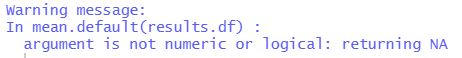
If you see anything I did faulty to receive these errors please let me know, as of now I am unable to see what I have done wrong.
The full R file for this module can be viewed and downloaded below. Any lines returning an error have been commented out in order to successfully compile the pdf.
All updated files for this site and for the modules can be viewed at my github page here.
Module 02: Test and Fix the Function
--January 22nd, 2021--
For this homework assignment, the task was to test a function posted in Canvas and identify it's possible errors.
I ran the function with the predetermined dataset (the vector object named assignment2) and R-Studio returned the following error:
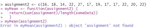
This error appears because the 'myMean' function calls upon two nonexistent data objects in its mean and length functions. It calls upon
an object named "assignment" in its mean function, and it calls upon an object named "someData" in its length function. For the myMean function to
properly compute the mean of "assignment2", it needs to call upon "assignment2" in both the mean and length functions within it.
I fixed the errors and wrote a new function named "myWorkingMean" that properly computes the mean of "assignment2", shown below:
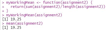
I also tested the result of "myWorkingMean" against R's built in "mean" function, and they returned the same values. This can be seen in the image above.
The full R file for this module can be viewed and downloaded below. The "myMean" function had to be commented out to successfully compile the file since it runs an error.
All updated files for this site and for the modules can be viewed at my github page here.
Module 01: First Assignment
--January 11th, 2021--
This is my first homework post for R programming in graduate school, very excited to be here!
My GitHub repository can be found here.
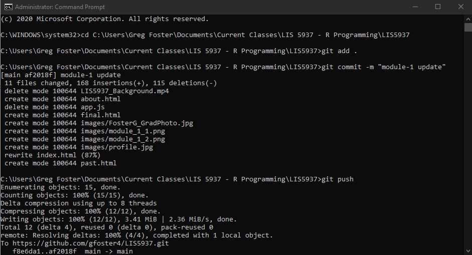
With the instruction in this week's module I successfully configured github so I can now use the command line to
update my repository, shown below.